How do we know our molecular simulation models are accurate? This is a very important aspect of all the work we perform on Folding@home. If we want to use simulations to model the dynamics and function of proteins, we need them to be reliable and accurate.
Force field models of proteins have been around for a long time (1). As computers have gotten faster and sampling methods more clever, the timescales we have been able to access have continued to grow (2). These models have been parameterized using mostly microscopic information, by comparing how well molecular mechanics (MM) energies compare to quantum mechanical (QM) energies. Therefore, as the timescales accessible by simulation have grown, it has been very interesting to test how well these models can predict macroscopic quantities like folding rates (3) and stabilities (the equilibrium between folded and unfolded states).
Exactly how to integrate macroscopic experimental measurements into the training of force fields—with their many microscopic parameters—remains an active area of research (4). The machine learning approach to this problem is to devise a score that measures the deviation between experimental measurements and their values predicted from simulations, and use optimization methods to adjust force field parameters to minimize the score.
But what is a good score? Suppose we perform a simulation and want to compare the results to some NMR measurements of (let’s say) chemical shifts, dj. A typical score is a “chi-squared” metric,
$$ \chi^2=\sum_{j=1}^N \frac{\left(d_j^*-d_j\right)^2}{\sigma_j^2}, $$
where dj* is a chemical shift calculated from the simulations, and σj2 is the expected variance, which reflects a combination of error in the measurements and the uncertainty in the chemical shift model we used to predict dj*.
While for some applications the chi-squared metric works well, in most cases we don’t really know the values of σj (they are hard to measure!) and instead want to infer them from the data.
For this reason,the Voelz lab has been pursuing a Bayesian inference approach through an algorithm we call BICePs (Bayesian Inference of Conformational Populations). In this approach, a simulation is considered a prior estimate p(X) of the population of different protein conformations, X, and a likelihood function that returns the probability of observing the experimental data given X and a particular value of σ. With a model for the prior distribution, p(σ), Bayes’ Theorem lets us sample the distribution of all the conformations X and σ:
$$ p(X, \sigma \mid D) \propto p(D \mid X, \sigma) \cdot p(X) p(\sigma) $$
$$ \text{posterior} \propto \text{likelihood} \cdot \text{priors} $$
There are some tricks to choosing good likelihood functions, and tricks to efficiently sample the distribution when there are lots of conformations and experimental measurements, but let’s skip all these details … What do we learn from all this sampling? A few things:
- We learn the posterior distribution of protein conformations X informed by the experimental measurements. In other words, a reweighted distribution that agrees (better) with experiment.
- We learn the posterior distribution of uncertainty parameters, σj, which are peaked at the most likely value. In other words, we have learned the uncertainties directly from the data.
And here’s the best part: through our sampling we also get a score that we can use for model selection, that we call the BICePs score. Without delving into too many details, we can calculate from all the samples the free energy cost of turning “on” the prior populations p(X), and the experimental restraints (i.e. the likelihood function). This is illustrated in the figure below.
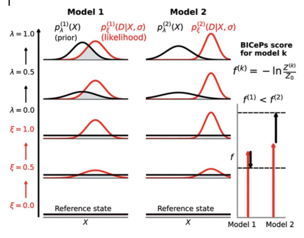
We tested this approach to model selection in a new paper from our group:
- Model Selection Using Replica Averaging with Bayesian Inference of Conformational Populations. Robert M. Raddi, Tim Marshall and Yunhui Ge, and Vincent A. Voelz. J. Chem. Theory Comput. 2025, 21, 12, 5880–5889. https://doi.org/10.1021/acs.jctc.5c00044
We used BICePs to reweight conformational ensembles of the mini-protein chignolin simulated on Folding@home (thank you folders!!!) in nine different force fields with TIP3P water, using a set of 158 published experimental NMR measurements (139 NOE distances, 13 chemical shifts, and 6 vicinal J-coupling constants for HN and Hα).
Below we show the result from reweighting populations of a Markov State Model built using the A99SB-ildn force field. Even though this force field favors the misfolded state, BICePs is able to correctly reweight the landscape.
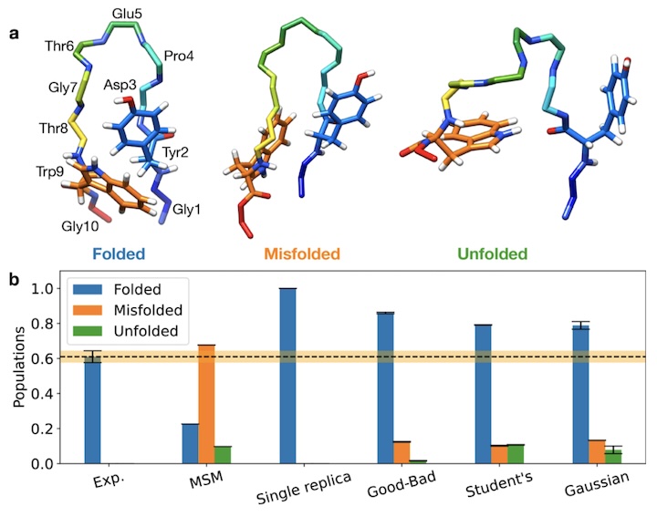
In all cases, reweighted populations favor the correctly folded conformation. And the BICePs score provides a metric to evaluate each force field. For the nine force fields tested (A14SB, A99SB-ildn, A99, A99SBnmr1-ildn, A99SB, C22star, C27, C36, OPLS-aa), we obtain results consistent with those of Beauchamp et al. (2012), who used a conventional χ2 metric to perform model selection for small polypeptides and ubiquitin simulated on Folding@home (!).
We are working on many ways to use the BICePs approach in the near future, including (1) Integrating the BICePs approach into automated pipelines for systematically validating models of conformational ensembles, and (2) using the BICePs score to variationally optimize parameters potential energy functions and forward models, as well as training generative machine learning models.
We have some manuscripts on the way that start to explore these ideas, so stay tuned!
References and Footnotes
- These models (typically) treat every atom as a point particle with partial charge, subject to bonded and nonbonded forces. We integrate the equations of motion using Newton’s laws (or stochastic variants thereof, like Langevin dynamics) to sample the ensemble of molecular configurations and their dynamics.
- In 1977 McCammon, Gelin and Karplus were able to simulate bovine pancreatic trypsin inhibitor (BPTI) for several picoseconds (1 ps = 10-12 s). Today, we can routinely generate milliseconds (1 ms = 10-3 s) of trajectory data for a small protein like BPTI.
- Snow, Christopher D., Eric J. Sorin, Young Min Rhee, and Vijay S. Pande. “How Well Can Simulation Predict Protein Folding Kinetics and Thermodynamics?” Annual Review of Biophysics and Biomolecular Structure 34, no. 1 (2005): 43–69. https://doi.org/10.1146/annurev.biophys.34.040204.144447.
- For a good review, see: Polêto, Marcelo D., and Justin A. Lemkul. “Integration of Experimental Data and Use of Automated Fitting Methods in Developing Protein Force Fields.” Communications Chemistry 5, no. 1 (2022): 38. https://doi.org/10.1038/s42004-022-00653-z.