The protein design field has been making great strides with the advent of new machine learning tools trained on large databases of protein structures and sequences.
While designs coming from these algorithms are good starting points, it is often necessary to improve upon them via an experimental procedure called affinity maturation. One first designs a library of proteins that are similar to the design, maybe differing from the original design by one or a few amino acids. Then one performs a high-throughput experimental screen to identify any members of this library that perform better than the original design, e.g. by binding more tightly to the intended target.
In a recent preprint, the Voelz lab shows how one can use massively parallel simulations on Folding@home to perform computational affinity maturation. As in the experimental procedure, they first create a library of proteins that are similar to the original design. However, instead of performing an experimental screen, they use expanded ensemble (EE) simulations to quantify the affinity of each member of the library to the intended target. The best binders from the library can then be tested experimentally to assess their potential utility relative to the original design.
Initial results are in reasonable agreement with experiment. Indeed, the Voelz lab’s EE method is better at identifying stabilizing and destabilizing mutations than a leading machine learning algorithm called Flex ddG (see figure below). These results means that one could accelerate the design/testing loop (and/or reduce its cost) by performing computational design, followed by a massive computation affinity maturation process, followed by experimental tests/screening on a smaller scale.
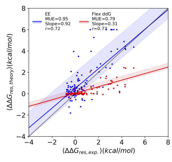
Prediction of average mutational effects at each position (called ∆∆G) for the Voelz lab’s EE method (blue) and the machine learning approach Flex ddG (red) at each position versus the average inferred experimental values. Solid lines are linear regression fits, with shaded regions corresponding to the the 95% confidence interval. The legend shows the mean unsigned error (MUE), slope, and Pearson r-value for each regression. The line of unity is shown in gray.