Dig deeper

Proteins are trying to get into their most “comfortable” position; that is, where they are at the best energy equilibrium with their environment. Many interactions drive what shape a protein will adopt. For example, some proteins contain areas that are hydrophobic (hate water), so those sections of the protein will end up away from the aqueous environment by hiding in the middle of the folded protein. There are many other factors that drive the protein, but there are several different analogies that can be used to explain the general process.

For one, think of a huge beach ball bouncing down the side of a steep mountain. The ball will bounce many times as it descends and will eventually stop. If you throw the beach ball down it again, there will be random variations in its path and it won’t end up at the same place. If you repeat that process many, many times, you can determine that there is a statistical pattern to the final resting points. You can also see a statistical scattering in the amount of time it takes for the ball to stop. Most of the time the ball will end up at the bottom of the mountain, but occasionally it may end up in another nearby depression and never reach the lowest possible stopping point. There is a significant statistical nature to atomic motions in proteins, much like the motion of the ball bouncing down the mountain. Normal folding is represented by all the times that the ball ends up at the lowest point. Misfolding is when the ball ends up somewhere else.

In some respects, it’s also similar to parallel-parking a car in a crowded street. At first, the car is exposed, and it usually takes several steps to park the car in the proper position. Sometimes it may be necessary to back out slightly and then try again. A protein does the same thing. If an observer watched a hundred similar cars being parked in that space, they would come to understand the common ways of parking and which methods work and which don’t.

Like both examples, it’s important for us to know about the motion of a folding protein, although we also want to know the intermediate steps along the way. Our simulation methods construct models of both of these properties. One aspect that makes Folding@home different from some other distributed computing projects (Rosetta@home, for example) is that we want to see how the car parks, not just the end state of seeing it parked. While that’s an important result, it doesn’t shed any light on how or why a protein sometimes misfolds. By attempting to study all of the possible paths that the bouncing ball can take down the mountain, we learn a lot about the question “How did we get here?” It also gives us the opportunity to introduce changes – such as drugs – into the process that modify the probability of misfolded results.

Two key aspects to our simulations are adaptive sampling and Markov State Models (MSMs). The two are used together and are very important as they allow us to run efficient simulations.

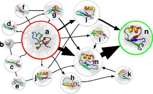
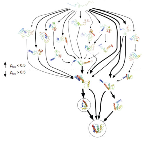
Protein folding is statistical in nature, so a protein can fold in many ways. We need a map to be able to see the bigger picture. Markov State Models (MSMs) are a way of describing all the conformations (shapes) a protein – or other biomolecule for that matter – explores as a set of states (i.e. distinct structures) and the transition rates between them. They also map out the protein’s motion and energy properties as it folds from one shape to another. Once we have all this information, we can observe the factors that influenced folding, which is especially important if the protein misfolds. Much of the theory underlying these methods is quite old but their use has been limited by the challenges inherent to identifying a reasonable set of states.

MSMs are particularly useful to us as they facilitate parallelization across many computer processors by allowing for the statistical aggregation of short, independent simulation trajectories. This replaces the need for single long trajectories, and thus has been widely employed by distributed computing networks such as Folding@home and GPUGRID. Further, through adaptive sampling, MSMs provide a way to increase the efficiency of simulation without introducing artificial biases or approximations. We’ve been making a lot of progress with developing Markov state model (MSM) methods for analyzing the data we generate with the help of the FAH community. Several Pande Group members include Drs. Xuhui Huang and Gregory Bowman have developed MSMBuilder, an open-source software package used to build, analyze, and visualize MSMs. Since its release in 2009, it’s been download over 1,600 times across five continents and has been used in at least 40 publications to date.

Formally, MSMs are a specific application of discrete-space master equations parameterized from simulation. They consist of two parts: a state space partitioning X, typically chosen to divide the system into a set of metastable states; and a master equation describing kinetics on X, represented by either a transition matrix T or rate matrix. Both the state space and master equation are found from molecular simulation. The precise manner in which this is done varies widely.

Here are two examples:

When researchers are using computers to study protein conformational dynamics (how the protein changes shape as it’s folding), the conventional approach for unbiased all-atom molecular dynamics is two-step. First, they run a set of simulations, and second, after the simulations have completed, they analyze the resulting data. The adaptive sampling Markov State Model approach involves breaking this paradigm by interleaving these two steps. Instead of building the model only after the data has been collected, it is instead built on the fly as the data is being generated. A feedback loop can then be set up where the current state of the model is used to inform the progress of further simulations.

Imagine, for example, that you were exploring a maze for the first time. Although you have no map, you do have a GPS which is able to track your progress and display the parts of the maze you’ve explored. One approach is to put the GPS in your purse and walk around blindly — bumping off walls — for as long as possible. Once you’re tired, you take out the GPS and analyze the path your trajectory took; by looking at your path on the GPS you’re able to see the structure of the maze and have effectively built a map. Unfortunately, you notice that you’ve wasted a lot of time stuck in various parts of the maze. Instead, the smarter strategy is to watch the GPS as you walk around — to try to build your map of the maze incrementally. Using your map, you’re able to identify when you’re “stuck” in a certain part of the maze, and to avoid re-exploring parts of the maze that you’re confident that you’ve already discovered.

In many ways, these two approaches to exploring a maze are analogous to the two approaches to collecting and analyzing molecular simulations. Due to the incremental nature of building the model on the fly in the adaptive sampling approach, it is possible to increase the efficiency of simulations.

To start a simulation project, we first must choose some initial conformations (a protein’s shape) to begin with. The heuristic methods we use so far include running high-temperature simulations, employing Rosetta’s Monte Carlo algorithm, and shooting off related MSMs of similar proteins. Once we have a set of conformations, each of them becomes the starting point for some simulations which together we call a Run. Within each Run, we launch many trajectories, each called a Clone. Thus, all of the Clones in a Run start from the same initial protein shape, but they have a different initial velocity, i.e. the atoms are given a different initial push in one direction or another. The Clones from a Run may find additional conformations, in which case that Run ends and several more Runs are started from them. This process continues with a lot of Runs branching out to other conformations, perhaps merging back together to a common shape with other Runs. In the end, we end up with a model with tens of thousands of different conformations, (terabytes of data!) and we can see all the shapes and energy states that the protein can take on while its folding towards its “native state”, the chances of all the transitions occurring, and how long it takes the protein to complete a transition from one conformation to another. More importantly, we can identify the places where the protein misfolds and gets stuck, which then leads to more research and models on how we can prevent this from happening. The more computers we have participating, the faster we can complete the Markov State Model.

Aren’t these the PRCG numbers?

Yes. Work Units are labeled with four distinct numbers in the format: Project (Run, Clone, Generation). We just described the first three; Project is the protein under study, a Run is a simulation started from a particular conformation, and Runs contain many Clones which have different initial velocities. Although Folding@home processes many different Projects, Runs, and Clones all at the same time, Clones themselves are serial in nature. They have to be simulated from start to finish, but it would be impractical for one computer to complete one by itself. Instead, your computer is given a piece of a Clone. We identify the piece using the Generation (Gen) number. One computer will start out with Generation 0, and when it finishes another computer is given Generation 1, etc. We cannot start Gen 1 until Gen 0 finishes, and there may be hundreds of Gens. This is why the Work Units have deadlines, and why speed is so important to us.

This approach can be powerful because not only is it very amendable to distributed computing, but the available computational resources can be used more efficiently. A protein spends most of its folding time “stuck” in an energetically-favorable position, with transitions – the processes largely of interest – taking place only rarely. Likewise, any straightforward simulation of protein folding will also waste valuable time generating data with little information content. However, using the adaptive sampling concept, the model can identify when the simulation is stuck, and then reinitialize new simulations starting from potentially more fruitful areas, avoiding the wasteful process of re-exploring areas that are already well understood.

In a recent paper, we compared MSMs to more traditional simulation methods. We compared some very long folding trajectories from the Anton supercomputer to an MSM built from the same folding data. Although our MSM “chops up” the simulation into a bunch of short trajectories, it was able to reproduce their simulations very well. Moreover, we also found that the MSM approach revealed new insights into the folding process (a new folding pathway) that was missing in ANTON’s more traditional approach.

MSMs and adaptive sampling have been used to study protein folding (1-8), functional dynamics (8-11), ligand-binding (11-14), and protein-protein interactions (15).

1. Jayachandran G, Vishal V, & Pande VS (2006) Using massively parallel simulation and Markovian models to study protein folding: Examining the dynamics of the villin headpiece. Journal of Chemical Physics 124:164902.
2. Bowman GR, Beauchamp KA, Boxer G, & Pande VS (2009) Progress and challenges in the automated construction of Markov state models for full protein systems. Journal of Chemical Physics 131(12):124101.
3. Noe F, Schutte C, Vanden-Eijnden E, Reich L, & Weikl TR (2009) Constructing the equilibrium ensemble of folding pathways from short off-equilibrium simulations. Proceedings of the National Academy of Sciences of the USA 106(45):19011-19016.
4. Bowman GR & Pande VS (2010) Protein folded states are kinetic hubs. Proceedings of the National Academy of Sciences of the USA 107(24):10890-10895.
5. Beauchamp KA, Ensign DL, Das R, & Pande VS (2011) Quantitative comparison of villin headpiece subdomain simulations and triplet-triplet energy transfer experiments. Proc Natl Acad Sci USA 108:12734-12739.
6. Bowman GR, Voelz VA, & Pande VS (2011) Atomistic folding simulations of the five-helix bundle protein (6-85). Journal of the American Chemical Society 133(4):664-667.
7. Voelz VA et al. (2012) Slow unfolded-state structuring in Acyl-CoA binding protein folding revealed by simulation and experiment. Journal of the American Chemical Society 134(30):12565-12577.
8. Lane TJ, Bowman GR, Beauchamp K, Voelz VA, & Pande VS (2011) Markov state model reveals folding and functional dynamics in ultra-long MD trajectories. Journal of the American Chemical Society 133(45):18413-18419.
9. Yang S, Banavali NK, & Roux B (2009) Mapping the conformational transition in Src activation by cumulating the information from multiple molecular dynamics trajectories. Proc Natl Acad Sci USA 106(10):3776-3781.
10. Morcos F, et al. (2010) Modeling conformational ensembles of slow functional motions in Pin1-WW. PLoS Computational Biology 6(12):e1001015.
11. Bowman GR & Geissler PL (2012) Equilibrium fluctuations of a single folded protein reveal a multitude of potential cryptic allosteric sites. Proc Natl Acad Sci USA 109(29):11681-11686.
12. Silva DA, Bowman GR, Sosa-Peinado A, & Huang X (2011) A role for both conformational selection and induced fit in ligand binding by the LAO protein. PLoS Computational Biology 7(5):e1002054.
13. Buch I, Giorgino T, & De Fabritiis G (2011) Complete reconstruction of an enzyme-inhibitor binding process by molecular dynamics simulations. Proc Natl Acad Sci USA 108(25):10184-10189.
14. Held M, Metzner P, Prinz JH, & Noe F (2011) Mechanisms of protein-ligand association and its modulation by protein mutations. Biophysics Journal 100(3):701-710.
15. Levin AM et al. (2012) Exploiting a natural conformational switch to engineer an interleukin-2 ‘super-kine.’ Nature 484(7395):529-533.

These questions were answered primarily by TJ Lane, Gregory Bowman, Robert McGibbon, Christian Schwantes, Vijay Pande, and Bruce Borden.